find a pairs trading strategy python

Away Anupriya Gupta

Pairs trading is supposedly one of the nearly popular types of trading strategy. In this scheme, normally a distich of stocks are listed in a commercialize-neutral strategy, i.e. it doesn't matter whether the market is trending upwards or down, the two open positions for each stock hedge against each other. The key challenges in pairs trading are to:

Choose a pair which will give you nice statistical arbitrage opportunities terminated time
Choose the entry/exit points

In this article along pairs trading, we will cover the pursual topics:

Correlation
Cointegration
How to choose stocks for pairs trading?
What is z-score?
Defining Entry points
Defining Going points
A simple Pairs trading strategy in Excel
Explanation of the model

Statistics play a life-and-death role in the first gainsay of deciding the match to trade. The pair is commonly chosen from the same basket of stocks, for example, Microsoft and Google (applied science domain) or ICICI danamp; Axis (Indian Banking) surgery Nifty Index and MSCI index (commercialize indices). Among each domain, in that respect are thousands of pairs are possible. The high-grade ones are those which are based on mathematical OR applied mathematics tests. We will see astir two statistical methods in the following surgical incision of pairs trading.

Correlation

Though not common, a few Pairs Trading strategies look up at correlation to find a suited pair to swap.

Correlation is quantified by the correlation coefficient ρ, which ranges from -1 to +1. The correlation indicates the level of correlation coefficient betwixt the two variables. The value of +1 way there exists a perfect positive correlation between the two variables, -1 means there is a perfect negative correlational statistics and 0 means there is no correlation.

A perfect positive correlation is when one variable moves in either up or pop direction, the other uncertain also moves in the same steering with the Saami magnitude while a perfect indirect correlation is when one protean moves in the upward direction, the other variable moves in the downwardly (i.e. opposite) direction with the duplicate magnitude.

The correlation coefficient for the two variables is presented aside

Correlation(X,Y) = ρ = COV(X,Y) / South Dakota(X).SD(Y)

where, cov (X, Y) is the covariance between X danamp; Y while SD (X) and SD(Y) denotes the standard departure of the respective variables.

If the correlation is graduate, enounce 0.8, traders may select that pair for pairs trading. This high phone number represents a strong relationship between the two stocks. So if A goes up, the chances of B sledding up are also quite high. Supported connected this supposition a market inert strategy is played where A is bought and B is sold; bought and sold decisions are made based on their independent patterns.

Just looking at correlation mightiness give you spurious results. For instance, if your pairs trading strategy is founded on the spread 'tween the prices of the two stocks, IT is possible that the prices of the two stocks retain increasing without ever so mean-regressive.

Spread = log(a) – nlog(b), where 'a' and 'b' are prices of stocks A and B respectively.

For each stock of A bought, you have sold n stocks of B.

Now, some 'a' and 'b' increases in much a way that the value of bedspread decreases. This will result in a loss since carry A is increasing at a rate lower than stock B and you are shortish along stock B.

Thus, one and only should be careful of victimization only correlation for pairs trading.

Let us now move to the next plane section in pairs trading basics, ie Cointegration.

Cointegration

The nigh common test for Pairs Trading is the cointegration prove. Cointegration is a statistical place of two operating room more time-series variables which indicates if a lineal combination of the variables is stationary.

Let United States of America understand this statement to a higher place. The two-time series variables, in this instance, are the log of prices of stocks A and B. Linear combination of these variables can be a linear equating shaping the prepared:

As you know, Bedcover = log(a) – nlog(b), where 'a' and 'b' are prices of stocks A and B respectively.

For each stock of A bought, you have sold n stocks of B.

If A and B are cointegrated so it implies that this equivalence above is stationary. A stationary cognitive operation has really valuable features which are compulsory to model Pairs Trading strategies. For instance, in that case, if the equation above is fixed, that suggests that the mean and variance of this equation corpse constant over time. So if we start with 'n', which is called the hedge ratio, so that spread = 0, the property of stationary implies that the expectation of spread will rest as 0. Any deviation from this expected value is a suit for statistical mental defectiveness, hence a grammatical case for pairs trading!

With the theory in mind, let us try to answer the doubt which you might be thinking of, in the next subdivision of Pairs trading basics.

How to choose stocks for pairs trading?

For whatever dyad of stocks, define the spread as below:

Spread = log(a) – nlog(b), where 'a' and 'b' are prices of stocks A and B severally.

Assumption: n, the elude ratio is constant.

Calculate 'n' using regression thusly that feast is as equal to 0 as possible. Hence, we regress the stock prices to calculate the elude ratio.

Theory: In regression, we fetch a term called the residuals which represents the distance of observed value from the curve fitting line operating theater estimated note value. These residuals tell us how much the true value of 'go around' deviates from 0 for the calculated 'n'. These residuals are unnatural so that we understand whether Oregon non they form a trend. If they do not form a trend, that agency the spread moves around 0 randomly and is stationary.

Run around the Dicky Fuller test on the spread (many complex and popular version is called Increased Dickie-seat Melville W. Fuller Test or ADF) values inserting the rate of 'n'.

Dickey Fuller test is a hypothesis test which gives pValue as the result. If this value is less than 0.05 surgery 0.01, we can say with 95% or 99% confidence that the signal is unmoving and we can choose this pair.

So far, we have discussed the challenges and statistics involved in selecting a pair of stocks for statistical arbitrage. We interpreted that past exploitation the cointegration tests, we commode say within a certain rase of confidence interval that the spread between the deuce stocks is a stationary signal. In other words, this signal is mean-reverting. The spread is defined as:

Spread = backlog(a) – nlog(b), where 'a' and 'b' are prices of stocks A and B respectively. For each stock of A bought, you have sold n stocks of B. n is premeditated aside regressing prices of stocks A and B.

Having already conventional that the equation above is mean reverting, we now involve to identify the extreme points Oregon threshold levels which when crossed by this signal, we trigger trading orders for pairs trading.

To be able to name these threshold levels, a statistical reconstruct called z-score is widely used in Pairs Trading. In the next section, on with the z-score, we will likewise do a brief dive in Moving averages which is another important component in Pairs trading.

What is z-score?

Plainly set up, given a Gaussian distribution of raw information points z-score is calculated so that the new distribution is a normal distribution with mean 0 and standard deviation of 1. Having much a distribution ~ N(0, 1) is very useful for creating threshold levels. For example, in pairs trading, we have a distribution of spread 'tween the prices of stocks A and B. We can commute these raw lots of spread into z-scores as explained to a lower place. This new distribution will have mean 0 and normal deviation of 1. It is easy to create threshold levels for this distribution much as 1.5 sigma, 2 sigma, 2.5 sigma, and so on.

How to calculate z-score?

z = (x – mean) / standard deviation, where x is a raw datum and z is the z-grade.

Mean and standard deviation can constitute rolling statistics for a full point of 't' days Oregon minutes or time intervals.

Moving average

We separate the data into subsets of sizing 't', where,'t' specifies a fixed time period for which the average is to be calculated. For example, to calculate the self-propelled average of the prices of stock A where 't' is 10 days, we start by calculating average afterward the first 10 days in the dataset. So we calculate moving average at 10th day, 11th day, 12th mean solar day etcetera. The average is moving or rolling. Soaring average and the textbook deviation is measured for 't' as 10 years in the table below.

The moving modal for 1-08-2001 or 11th entry would not take into account statement the prime data point, that is, stock A prices happening 18-07-2001.

Using these concepts of squirming averages and z-score we create the entry points for Pairs Trading.

Defining Entry points

Let U.S.A denote the Spread atomic number 3 s. Thus,

Spread = s = log(a) – nlog(b)

Compute z-score of 's', exploitation rolling mean and criterial deviation for a time period of 't' intervals. Save this as z.

Delimit threshold as anything 1.5-sigma, 2-sigma. This parametric quantity will change as per the backtesting results without risking overfitting to data.

When Z-make crosses upper threshold, go SHORT:

Sell breed A

Buy stock B

When z-scotch crosses the lower door, XTC LONG:

Buy stock A

Sell stock B

Maintain the hedge ratio to calculate the stock quantity

We make now understood Entering points in Pairs trading. Now we will move on to the other end, exit points.

Defining Exit points

STOP LOSS

Stop loss is defined for scenarios when the expected cause not happen. For example, if we chose entry signals at 2-sigma, we are expecting that the spread volition revert back to ungenerous from this room access. However, information technology is possible that spread continues to detonate. Say it reaches 2.5-sigma and you incurred losses. To prevent promote losings, you place Stop Loss at say 3-sigma.

To boot to placing a pre-defined give up-loss criterion such as 3-sigma or extreme magnetic variation from the mean, you can break along the co-integration value. If the conscientious objector-integration is broken during the pair is ON, the strategy warrants slip the positions since the rudimentary hypothesis is nullified.

TAKE PROFIT

It is defined as scenarios where you take profits in front the prices move in the other charge. For instance, say you are LONG on the spread, that is, you have brought standard A and sold sprout B as per the definition of spread in the article. The expectation is that spread leave regress back to mean operating theatre 0. In a juicy situation, the mean would cost approaching to zero or very close to it. You can keep Take Earnings scenario as when the mean crosses zero for the premier time after lapse from threshold levels.

There can be many shipway of defining get hold of profit depending on your gamble appetence and backtesting results.

What ofttimes works is your experience and a broad range of equipotent skillsets that earmark you to grasp a hold of the complete scenario before jump to conclusions and help you understand much. Like we mentioned, your appetency for jeopardy and backtesting results will mold for you. Automation and practical applications are the keys here. Anto, who had been trading for 10 years, evolved his skillsets and altered to the growing markets with the Executive Broadcast in Recursive Trading (EPAT) and is happily trading in this field.

Let us try to recapitulation what we have understood so far. Pairs Trading is a trading strategy that matches a long position in one stock/asset with an offsetting position in another stock/asset that is statistically related. Pairs Trading can be named a mean backsliding strategy where we bet on that the prices bequeath retrovert to their historical trends.

So far, we suffer asleep through the concepts and now let us try to create a simple Pairs Trading scheme in Excel.

A simple Pairs trading strategy in Excel

This excel fashion mode testament serve you to:

Learn the application of have in mind regress
Understand of Pairs Trading
Optimize trading parameters
Understand probative returns of statistical arbitrage

Wherefore should you download the trading role model?

As the trading logic is coded in the cells of the sheet, you can improve the apprehension aside downloading and analyzing the files at your own convenience. Not just that, you can dabble the numbers to get wagerer results. You might find suited parameters that provide high profits than specified in the article.

Account of the poser

In this example, we study the MSCI and Nifty pair As both of them are stock market indexes. We follow up mean reversion strategy on this pair. Mean reversion is a property of stationary time serial. Since we claim that the pair we undergo chosen is mean reverting we should test whether it follows stationarity.

Plotting of the exponent ratio of Nifty to MSCI makes it appear to be mean reverting with a mean value of 2.088 simply we utilise Dicky Fuller Essa to test whether it is stationary with a statistical significance. The results under Cointegration output table shows that the Leontyne Price series is nonmoving and hence mean-reverting. Dicky Fuller Try out statistic and a significantly abject p-value (danlt;0.05) confirms our assumption. Having determined that the mean reversion holds true for the chosen pair we proceed with specifying assumptions and stimulation parameters.

Assumptions

For simplification purpose, we snub tender-ask spreads.
Prices are uncommitted at 5 minutes intervals and we trade at the 5-second closing price only.
Since this is separate data, squaring remove of the position happens at the remnant of the candle i.e. at the price available at the end of 5 minutes.
Only the regular session (T) is traded
Dealings costs are $0.375 for Nifty and $1.10 for MSCI.
The security deposit for each trade is $990 (approximated to $1000).

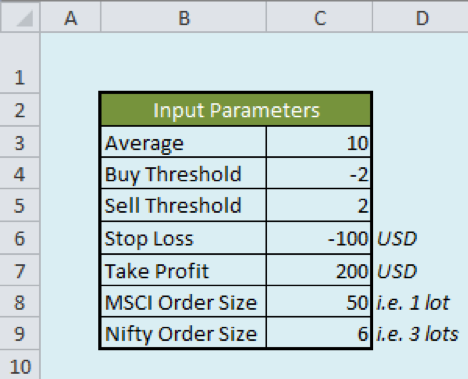
Input parameters

Please note that all the values for the input parameters mentioned below are configurable.

Average of 10 candles (1 candle is equivalent to all 5-minute price) is considered
A "z" score of +2 is considered for buy and -2 for selling
A stop loss of $100 and profit limit of $200 is set
The order size for trading MSCI is 50 (1 lot) and for Nifty is 6 (3 lots)

The marketplace data and trading parameters are included in the spreadsheet from the 12th row onwards. So when the reference is made to column D, it should be overt that the reference commences from D12 forward.

Explanation of the columns in the Excel Model

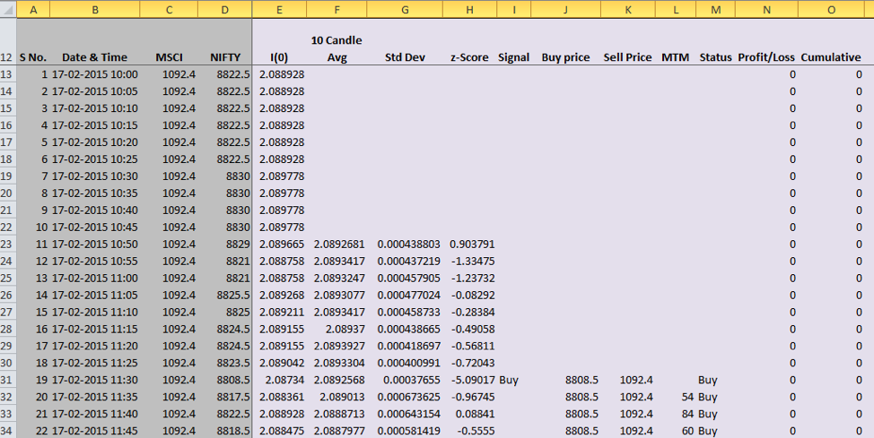
Column C represents the price for MSCI.

Column D represents Nifty price.

Column E is the logarithmic ratio of Nifty to MSCI.

Column F calculates 10 taper norm. Since 10 values are needed for average calculations, there are no values from F12 to F22.

The formula =IF(A23dangt;$C$3, AVERAGE(INDEX($E$13:$E$1358, A23-$C$3):E22), "") substance that the mean should be calculated only the data sample available is more than than 10 (i.e. the value specified in cell C3), otherwise the cellphone should be blank shell.

Reckon cell F22. Its corresponding cell A22 has a value of 10. Since A22dangt;$C$3 fails, the entry therein jail cell is blank. The next cell F23 has a economic value since A23dangt;$C$3 is true. Let's move to the future pillar.

In column G, the formula, AVERAGE(INDEX($E$13:$E$1358, A23-$C$3):E22) calculates the average esteem of last 10 (as mentioned in cell C3) candles of column E data. Similar logic holds for column G where the authoritative deviation is calculated.

The "z" score is calculated in the column H. Formula for calculating "z" scotch is z= (x-μ)/(σ). Present x is the sample (Column E), μ is the think of value (Column F) and σ is the standard deviation (Column G).

Pillar I represents the trading signal. A mentioned in the input parameters, if "z" score goes below -2 we buy and if it goes higher up +2 we sell. When we say buy, we have a long position in 3 slews of Nifty and have a short position in 1 lot of MSCI. Similarly, when we say deal, we have a long lieu in 1 lot of MSCI and have a short position in 3 lots of Nifty so squaring off the position. We have one open post all the time.

To understand what this substance, consider two trading signals "buy" and "sell". For the "buy" signal, as explained before, we buy 3 lots of Keen future and dead 1 muckle of MSCI future. Once the position is taken, we track the position using the Status tower, i.e. column M. In each new run-in while the position is continuing, we check whether the stop release (as mentioned in cell C6) or take profit (As mentioned in cell C7) is off. The block up loss is given the value of USD -100, i.e. loss of USD 100 and take earnings is given the value of USD 200 in the cells C6 and C7 respectively.

Spell the position does non bang either stop loss or return profit, we proceed with that trade and ignore all signals that are appearing in column I. Once the trade hits either the stop passing or take profit, we again start look at the signals in pillar I and subject a unaccustomed trading position equally soon arsenic we birth a Buy or Sell signal in editorial I.

Column M represents the trading signals based along the input parameters specified. Column I already has trading signals and M tells the States about the status of our trading put back i.e. are we long or curtal or set-aside the profits or exited at the stop loss. If the trade is not exited, we contain forward the berth to the close candle by repetition the value of the condition column in the former candle. If the price campaign occurs in such a way that it breaches the given TP or SL then we square up our billet thus denoting IT away "TP" and "Shining Path" respectively.

Column L represents Mark out to Market. It specifies the portfolio position at the end of time period. As nominal in the input parameters we trade 1 lot of MSCI and 3 lots of Nifty. Thusly when we trade our position is the appropriate cost difference (depending on whether we are bought or sold-out) multiplied by the number of lots.

Column N represents the earnings/red ink condition of the trade. P/L is calculated only when we have squared off our position. Column O calculates the accumulative profit.

Outputs

The output table has some performance metrics tabulated. Loss from all loss-making trades is $3699 and profit from trades that hit TP is $9280. So the total P/L is $9280-$3699=$5581. Loss trades are the trades that resulted in losing money on the trading positions. Fat trades are the successful trades finish in gaining cause. Average profit is the ratio of total profit to the total number of trades. Net average profit is calculated later on subtracting the transaction costs which amounts to $91.77.

Now information technology is your turning!

Primary, download the model
Modify the parameters and analyse the backtesting results
Run the model for other diachronic prices
Qualify the pattern and scheme to add new parameters and indicators! Play with logic! Explore and study!

Comment below with your results and suggestions

Summary

Thus, we have implicit the concept behind Pairs trading strategy, including correlation and cointegration. We also took a deal Z-score and defined the entry and exit points when we are executing a pairs trading strategy. We also created an Excel model for our Pairs Trading scheme!

Learn how to implement pairs trading/statistical arbitrage strategy in FX markets through with a project work including live examples. If you want to dig deeper and try to witness suitable pairs to apply the scheme, you can go through the blog on K-Means algorithm.

If you want to learn single aspects of Algorithmic trading then gibe out our Executive Programme in Algorithmic Trading (EPAT). The course covers training modules like Statistics danamp; Econometrics, Financial Computer science danAMP; Technology, and Algorithmic danamp; Quantitative Trading. EPAT is designed to equip you with the right skill sets to be a successful bargainer. Enroll directly!

Disclaimer: Whol information and information provided in this clause are for informational purposes entirely. QuantInsti^® makes no representations every bit to accuracy, completeness, currentness, suitability, or rigor of any information in this article and will not be nonexempt for any errors, omissions, or delays in this information or any losses, injuries, operating theater damages arising from its display surgery use. All selective information is provided on an as-is foundation.